Machine-Learning Introduction:
Using SciKit-Learn
My first experience with Machine Learning algorithms comes from having to use OpenCV's implementation of the K Nearest Neighbors algorithm to read the numbers on the Sudoku puzzle. I've learned a lot about the theory behind various Machine Learning algorithms from watching many hours of mathematicalmunk's youtube channel. Experimenting with the algorithms in SciKit-Learn has certainly led to a deeper understanding.
Clustering
SciKit-Learn is an awesome Python module that enables you to easily use Machine Learning algorithms if you understand the basics of how they work. All of the images I'm about to show you are from examples that you can download from SciKit - Learn's website and try for yourself. I didn't write these algorithms, I'm just going to use them to explain some of the basics of Machine Learning.
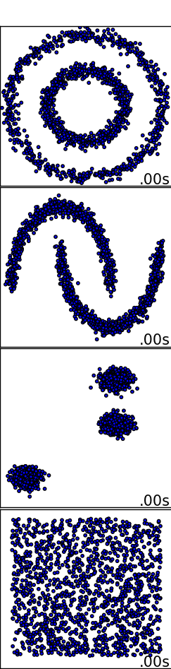
Let's say you had 4 different sets of some 2-dimensional data and you wanted the computer to find patterns within each set of data. Specifically in this case we want the data to be classified into groups. When a human looks at these four different examples they would easily be able to define 2 different circular groups in the first dataset, 2 different crescent groups in the next set, 3 groups in the next set, and finally in the last set there is no real pattern so all of the data belongs to the same group.
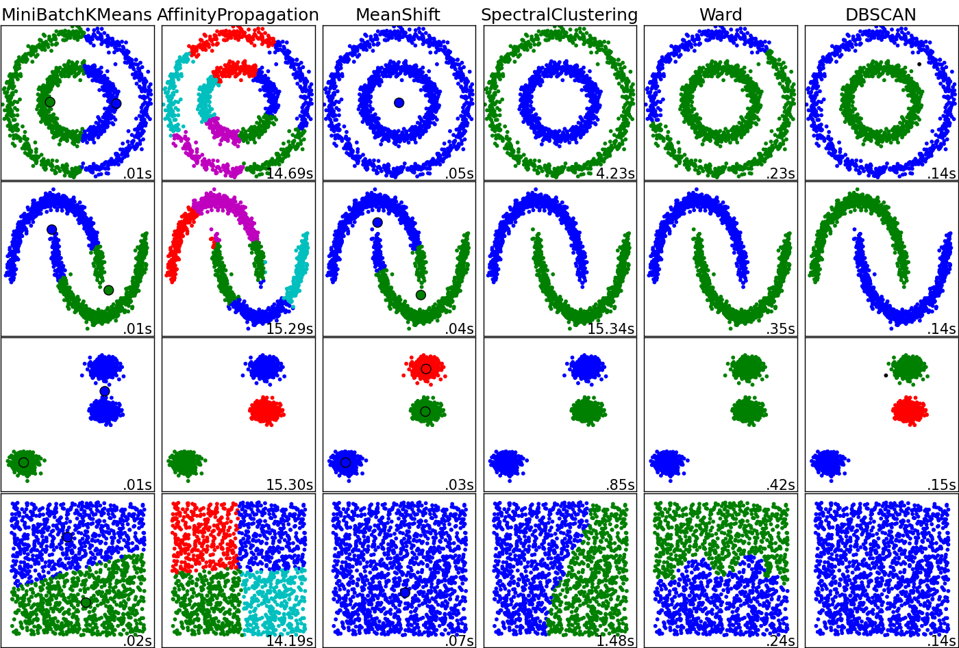
If you instead wanted the computer to try to figure out how to group the data you could use a process called clustering, which is an unsupervised machine-learning process. The results of six different clustering algorithms are shown below. The color differentiates between the different groups that the algorithm has found.
For some of these algorithms, such as MiniBatchKMeans, you must tell it how many groups it needs to find. So in this example we would have input a K value of 2. But you can see from the results for MiniBatchKMeans that it didn't do a very good job on any of the datasets. Maybe if we had input a K value of 3 it would have classified the 3rd data set correctly. On the right side we have DBSCAN which seems to have gotten every dataset correct.
However this example is somewhat deceiving. With higher dimensional data you might find different results where the algorithms that appear to do poorly are in fact quite good.
Classification
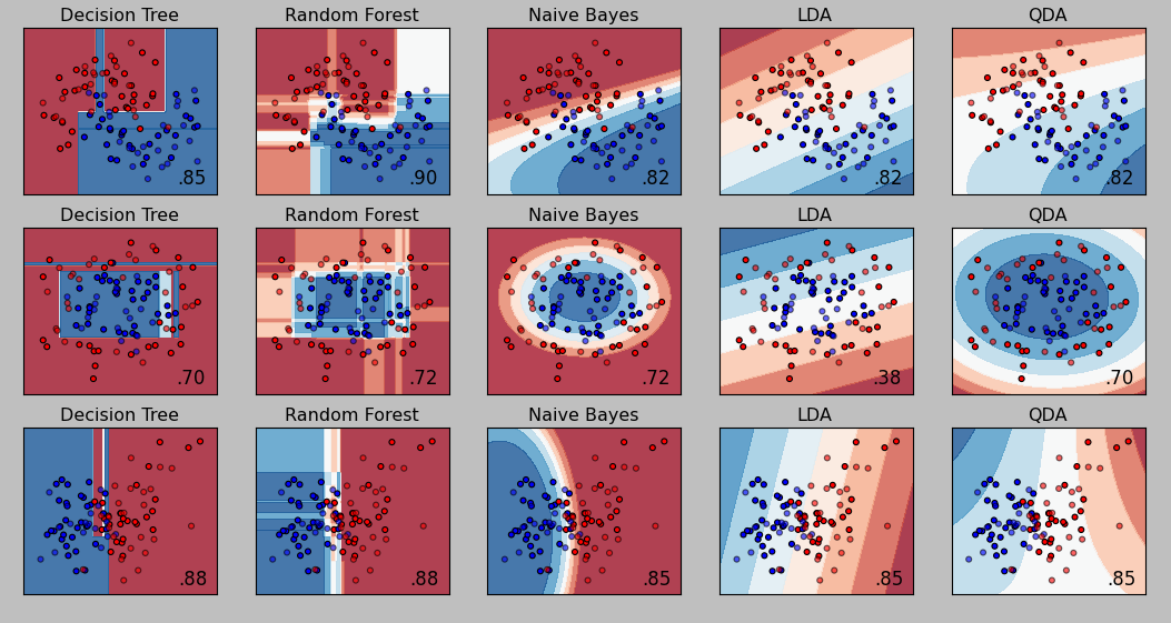
These next algorithms are called classifiers and they are a supervised machine-learning process. These classifier algorithms are called a supervised process because you train them with training data first and then you test them on different testing data. In the unsupervised algorithms there was no training process, you only have to give it your testing data and it will return a result.
In the image below on the left side there are red and blue dots. Some of the dots are a lighter red/blue and some of the dots are a darker red/blue. The darker dots represent the training data that is first fed into the algorithm. Then the algorithm creates the red and blue areas which represent the probability of a testing data point being classified as red or blue. So if light red point falls in a blue area it will be incorrectly classified. If the light red point falls in a red area it will be correctly classified, and so on...
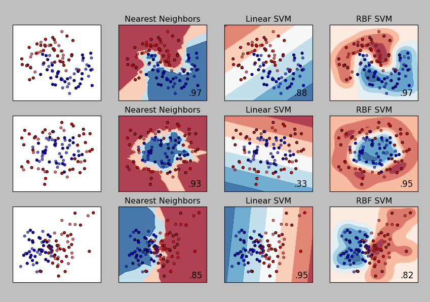
So these classifier algorithms are still involved with grouping data, the difference is that groups are already defined and the classifier just has to decide what existing group the new testing data should be grouped with. Here are some additionaly classifiers below. Similar to the clustering algorithms, this example may be somewhat deceiving. With real-world data sets and more dimensions you may find different results.
Regression
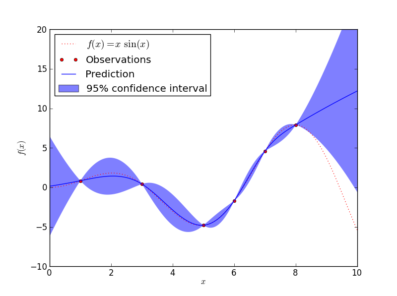
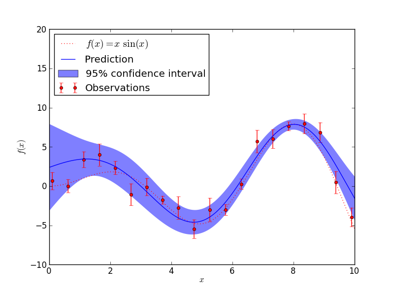
Many of the classifier algorithms can also do regression. For example, lets say we use the K Nearest Neighbors algorithm on a very simple dataset. If we set K = 3 that means that when we choose a new test point we want to find the 3 nearest neighbors to that new test point. These neighbors come from the test data that we have already supplied to the algorithm. So the results from running KNN in Classification mode and Regression mode on the same data might look like this:
>>>
Classification
retval: 20.0
results: [[ 20.]]
neighResp: [[ 20.  20.  10.]]
dists: [[  3.   9.  10.]]

Regression
retval: 16.6666660309
results: [[ 16.66666603]]
neighResp: [[ 20.  20.  10.]]
dists: [[  3.   9.  10.]]
>>>
In both cases the 3 nearest neighbors have values of 20, 20, and 10. So in classification mode the 20s win and the test data gets classified as a 20. In the case of regression we get a result of (20 + 20 + 10)/3 = 16.66. Classification is used when the response values are meant to be purely a label for the group, whereas Regression is used if the response values are real numbers.
Regression Analysis is defined as finding the relationship between a dependent variable and the independent variables. In the previous example the test data make up the independent variables and the response value is the dependent variable. Regression is very important in basic statistics, and basic statistics is very important in machine-learning. SciKit - Learn also has some helpful graphing tools for basic statistics as well.
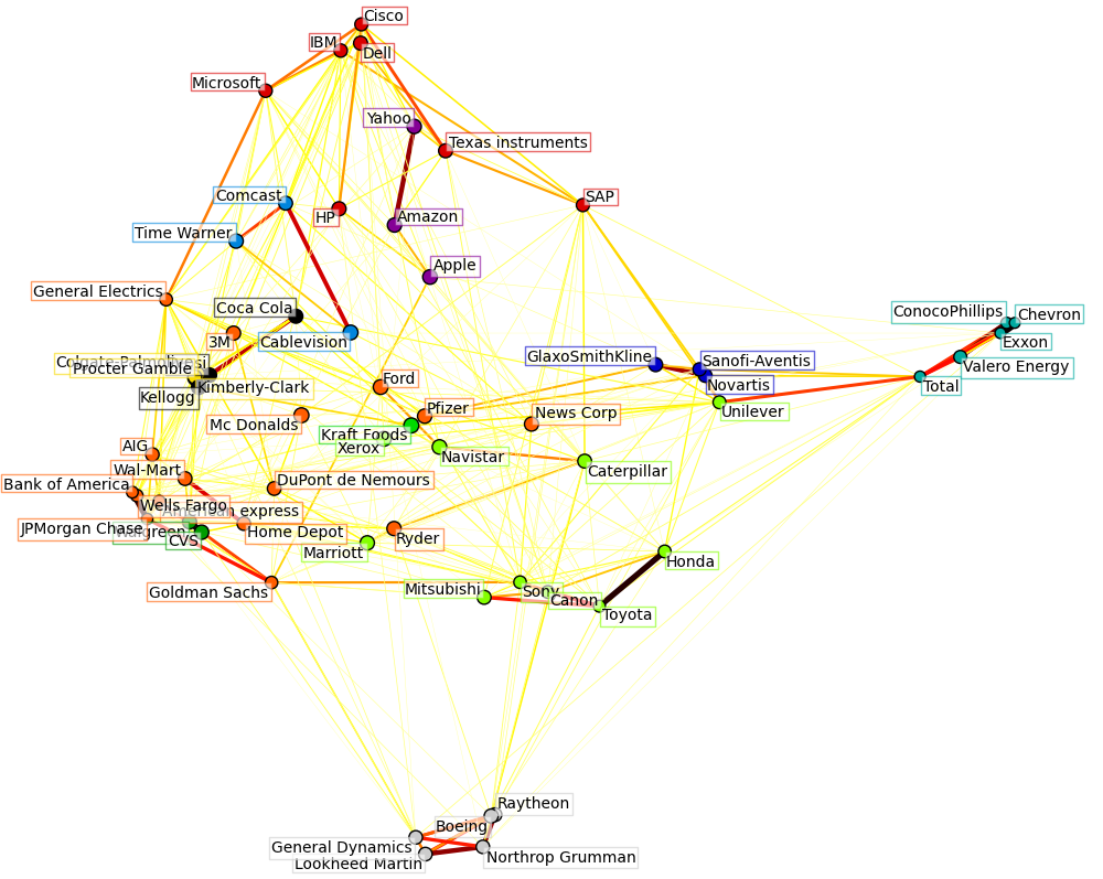
Covariance Analysis
Covariance Analysis studies the strength of a relationship between two variables. A good example of this would be to find the relationship between the the changes in stock prices for various companies.
Dimension Reduction
Sometimes it can be useful to take high-dimensional data and reduce it down to fewer dimensions. This is especially useful for visualizing results in 2-dimensions. Take this example of digit classification where the image of the digit is highly dimensional. An image of a digit can be stored in a 2D array. This may be counter intuitive at first, but if you want to represent the entire image of the digit as a single point (so that one can compare it to other digits) then every pixel represents a new dimension. Fortunately there are algorithms that can reduce dimensions for us, but obviously there is some loss to the accuracy of the results because the data has been changed.

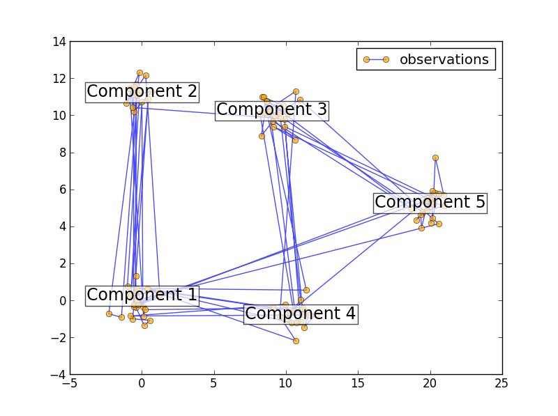
Markov Chains
Markov Chains are actually fairly simple mathematically and conceptually as well. They are used to model problems where you have a set of states that an object can be in. Let's say the number of possible states, N, is equal to 5. Next you define the probability that the object starts in each of the states. This would have to be a 1 x N array that sums to a probability of 1. The last step is to define all of the probabilities that any state will move to any state. This would be an N x N array called the Transition Matrix. If 'i' represents the row and 'j' represents the column then the ij-th element represents the probability that an object in the i-th state would move to the j-th state. Therefore each row in this matrix also has to sum to a probability of 1.
# Initial population probability
start_prob = np.array([0.6, 0.3, 0.1, 0.0, 0.0])
# The transition matrix
trans_mat = np.array([[0.5, 0.2, 0.0, 0.1, 0.2],
                      [0.3, 0.5, 0.2, 0.0, 0.0],
                      [0.0, 0.0, 0.6, 0.3, 0.1],
                      [0.2, 0.0, 0.2, 0.5, 0.1],
                      [0.1, 0.1, 0.2, 0.0, 0.6]])
Notice that according to this Transition Matrix an object can loop from its own state back into itself. You can see that anywhere a zero appears in the Transition Matrix you will find no connecting lines between those two states.